드디어 4주차이다.
4주차에서는
- Reading Files with Open
- Pandas
- Numpy in Python
을 공부한다.
Reading Files with Open
시작하기 전에, 구글 드라이브와 구글 colab 을 연동하는 방법을 해봐야겠다. External data: Local Files, Drive, Sheets, and Cloud Storage 링크를 참고했다.
from google.colab import drive
drive.mount('/content/drive')
를 시행하면, Mounted at /content/drive 라고 확인이 된다.
테스트로 다음 코드를 시행해보자.
with open('/content/drive/My Drive/foo.txt', 'w') as f:
  f.write('Hello Google Drive!')
내 구글드라이브에 바로 foo.txt 에 파일이 저장된다.
example1 = "/content/drive/My Drive/DataScience/Python4DS_AI_Dev/exampleText.txt"
fileExample=open(example1,"r")
fileContent = fileExample.read()
print(fileContent)
텍스트 속에 있던 내용인 first line 1 second line 2 third line 3 가 출력된다.
with open(example1, "r") as file1:
    fileContent = file1.read()
    print(fileContent)
는 first line 1 second line 2 third line 3 fourth line 4 fifth line 5 를 출력한다.
with open(example1, "r") as file1:
    fileContent = file1.readlines()
    print(fileContent)
는 ['first line 1\n', 'second line 2\n', 'third line 3\n', 'fourth line 4\n', 'fifth line 5'] 를 출력한다.
with open(example1, "r") as file1:
    for line in file1:
      print(line)
는 각각의 line 에 있는 값들을 출력한다. first line 1 second line 2 third line 3 fourth line 4 fifth line 5
with open(example1, "r") as file1:
  file_element = file1.readlines(1)
  print(file_element)
  file_element = file1.readlines(1)
  print(file_element)
  file_element = file1.readlines(1)
  print(file_element)
  file_element = file1.readlines(1)
  print(file_element)
  file_element = file1.readlines(1)
  print(file_element)
내 예시의 경우는 ['first line 1\n'] ['second line 2\n'] ['third line 3\n'] ['fourth line 4\n'] ['fifth line 5'] 를 차례로 출력하는데, 파일이 영상에 나오는 파일의 구조와 다른게 아닐까 하는 생각이 든다.
Writing Files with Open
with open('/content/drive/My Drive/DataScience/Python4DS_AI_Dev/exampleWrite.txt', 'w') as f:
  f.write('This is the first line \n')
  f.write('This is the second line')
는 exampleWrite.txt 파일에 두 줄에 걸쳐 문장을 적어준다.
lines = ["Question: What date is it today?\n","Answer: It is May 20th\n","How's the weather like in Texas?\n","It is hot\n"]
with open('/content/drive/My Drive/DataScience/Python4DS_AI_Dev/exampleQnA.txt', 'w') as f:
  for line in lines:
    f.write(line)
는 아래와 같은 텍스트를 출력한다.
Pandas
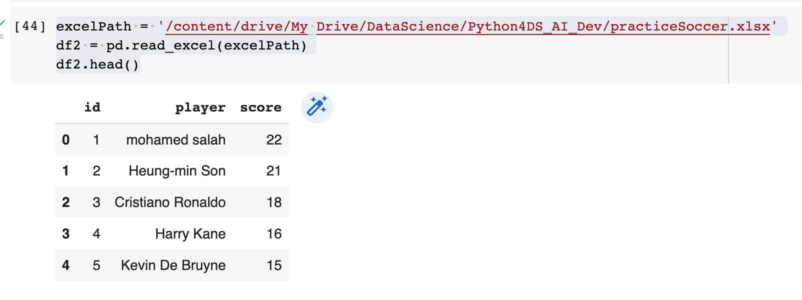
pandas 는 csv 와 같은 엑셀 파일 형태를 불러온다.
df.head() 는 첫 다섯 개의 행을 보여준다.
csv 경우와 마찬가지로 excel 을 이용해도 다음과 같이 된다.
DataFrames

데이터 프레임을 만들 수도 있다.

위의 데이터 프레임에서 날짜와 최고기온만 가져오고 싶으면 다음의 코드를 사용하면 된다.
dateMaxCel=weatherFrame[['date','celciusMax']]
dateMaxCel
Pandas: Working with and Saving Data
유니크한 원소의 개수를 구하려면
dateMaxCel['celciusMax'].unique()는 array(['33', '28', '29'], dtype=object) 를 출력한다.
최근 6일 중에서 영상 30도 이상이었던 날만 고른다고 하자.
weatherFrame['celciusMax'] = weatherFrame['celciusMax'].astype(float)
weatherFrame2 = weatherFrame[weatherFrame['celciusMax']>=30]
weatherFrame2.to_csv('/content/drive/My Drive/DataScience/Python4DS_AI_Dev/practiceHotDays.csv')
weatherFrame2
그러면, csv 파일이 아래와 같이 출력이 된다.

slicing : loc() 또는 iloc() 함수를 사용한다.

추가적으로, set index 를 정한 이후에, index 를 이용해서도 행의 slicing 이 가능하다.

weatherFrame.loc[3,'celciusMax'] 는 가능한데, weatherFrame.loc[3,4] 는 에러가 난다.
Numpy in Python
1차원 Numpy
nd array 는 list 와 유사하다.
import numpy as np
x = np.array([2,4,6,8,10])
x[1]
는 4를 출력한다.
type(x)는 numpy.ndarray 를 출력한다.
x.size는 5를 출력한다.
x.ndim는 (5,) 를 출력한다.
y=np.array([2.1,3.4,5.0,4.4])에 대해, type(y) 는 numpy.ndarray 출력하고, y.dtype 는 dtype('float64') 를 출력한다.
Indexing and Slicing
z = np.array([9,8,9,6,7])
z[1]=9
z
는 변화된 array([9, 9, 9, 6, 7]) 를 출력한다.
w = z[2:4]
w
는 array([9, 6]) 를 출력한다.
z[1:3]=5,6
z
는 변화된 array([9, 5, 6, 6, 7]) 를 출력한다.
기본 연산
벡터 덧셈과 뺄셈
numpy 를 사용하지 않은 벡터의 연산은 다음과 같다.
vec1=[1,0]
vec2=[0,1]
vec3=[]
for x,y in zip(vec1,vec2):
  vec3.append(x+y)
vec3
numpy 를 사용하면 코드가 간소화된다.
vec4=np.array([1,0])
vec5=np.array([0,1])
vec6=vec4+vec5
vec6
위 코드의 출력값은 array([1, 1]) 이다.
Scalar 만큼 곱하기
vec7=2*vec4
vec7
는 array([2, 0]) 를 출력한다.
두 개의 numpy array 곱하기
vec8=np.array([2,3])
vec9=np.array([4,3])
vec10=vec8*vec9
vec10
는 array([8, 9]) 를 출력한다.
Dot Product
vec11=np.array([3,4])
vec12=np.array([5,1])
vecDot = np.dot(vec11,vec12)
vecDot
는 19 (=3 x 5 + 4 x 1)를 출력한다.
numpy array 에 상수 더하기
vec13 = np.array([4,3,2,4,5,-2])
vec14 = vec13+2
vec14
는 array([6, 5, 4, 6, 7, 0]) 를 출력한다.
Universal Functions
평균을 구할 수 있다.
maxTemp=np.array([34,28,29,28,29,28,30,32])
avg_maxTemp = maxTemp.mean()
avg_maxTemp
는 1/7 x (34+28+29+28+29+28+30+32) 값인 29.75 를 출력한다.
최댓값도 구할 수 있다.
maxOfmaxTemp = maxTemp.max()
maxOfmaxTemp
는 34를 출력한다.
numpy 는 pi 와 같은 값을 출력하기도 한다.
x=np.array([-np.pi,-np.pi/2,0,np.pi/2,np.pi])
y=np.cos(x)
y
는 array([-1.000000e+00, 6.123234e-17, 1.000000e+00, 6.123234e-17, -1.000000e+00]) 를 출력하고,
cosine 그래프를 -2*\pi 와 2*\pi 사이에 그려보면,
import matplotlib.pyplot as plt
x = np.arange(-2*np.pi,2*np.pi,0.1)   # start,stop,step
y = np.cos(x)
plt.plot(x,y)
코사인 그래프가 잘 그려진다.
x2 = np.linspace(-2*np.pi,2*np.pi,100)
y2=np.cos(x2)
plt.plot(x2,y2)
이렇게 해도 위 그래프와 동일한 결과가 나온다.
이차원 Numpy
A=np.array([[11,12,13],[21,22,23]])
A
는 array([[11, 12, 13], [21, 22, 23]]) 를 출력한다.
11 12 13
21 22 23
의 2 x 3 형태의 행렬을 닮았다.
A.ndim 은 2 를 출력하고, A.shape 은 (2,3) 을 출력하고, A.size 는 6을 출력한다.
A[0][0] 은 11 을 출력한다. A[0,1] 은 12 를 출력한다.
A[1,0:2] 는 21,22 를 출력한다.
행끼리 더할 수 있다.
scala 만큼 곱하는 연산도 가능하다.
B=np.array([[1,1],[1,1]])
C=np.array([[1,3],[4,1]])
B+2*C
는 array([[3, 7], [9, 3]]) 를 출력한다.
행렬의 각 원소끼리 곱할 수 있다.
D=np.array([[1,1],[2,2]])
E=np.array([[1,2],[3,4]])
D*E
는 array([[1, 2], [6, 8]]) 를 출력한다.
행렬의 곱도 가능하다.
F=np.array([[1,1],[2,2],[3,3]])
G=np.array([[1,2,3],[3,2,1]])
np.dot(F,G)
는 array([[ 4, 4, 4], [ 8, 8, 8], [12, 12, 12]]) 를 출력한다.
'머신 러닝' 카테고리의 다른 글
| [머신러닝 코세라 강의] (2주차) "Cost Function & Gradient Descent" Machine Learning (by Andrew Ng) (0) | 2022.05.26 |
|---|---|
| [데이터과학 코세라 강의] (1주차) 파이썬을 이용한 머신러닝 (0) | 2022.05.22 |
| [데이터과학 코세라 강의] (3주차-2) 데이터 과학을 위한 파이썬 (0) | 2022.05.21 |
| [데이터과학 코세라 강의] (3주차-1) 데이터 과학을 위한 파이썬 (0) | 2022.05.20 |
| [데이터과학 코세라 강의] (2주차) 데이터 과학을 위한 파이썬 (0) | 2022.05.19 |